Not all measurements are worth collecting: information value vs. collection cost in the RAN

The instinct to collect everything

Minimization of Drive Tests has been in the 3GPP specifications since Release 10. It lets the network ask ordinary UEs to report radio measurements, with location where available, instead of sending a van with test equipment around the city. Immediate MDT collects from connected UEs and reports at once. Logged MDT lets idle or inactive UEs record measurements and hand them over later, when they connect again.

It works, and it is cheap compared with a drive test. That is exactly the problem. When collection is cheap, the natural answer to "should we measure here" is always yes. Networks end up with trace collection entities full of reports that nobody looked at, from areas the model already understood, while the places where the model was really unsure got the same coverage as everywhere else.

This post argues for a different question. Not "can we measure here" but "what would this measurement change".

What collection really costs

The costs of MDT are spread out and easy to overlook. Start with the UE. Every measurement configuration means extra measurement activity and extra reporting, and both draw on the battery. Logged MDT also uses UE memory, and the UE keeps the log for a limited time; if the network never retrieves it, the effort was wasted.

Then the radio interface. Reports travel over RRC signalling. Frequent reports from many UEs add load on the control plane at the very moment the cell is busy, which is often when you wanted the data.

Then the network side. Trace records cross the backhaul, land in a trace collection entity, get stored, parsed and processed. At scale this is real compute and real storage, and it has an energy cost of its own. A measurement campaign that runs to find a few percent of energy saving can eat a noticeable part of that saving in the collecting.

None of this argues against measuring. It argues for putting the cost on the same page as the benefit.

What a measurement is worth

The benefit of a measurement is the decision it improves. A coverage model that already knows the signal strength on a highway to within a dB does not get better with another thousand samples from the same road. The same thousand samples from a new residential area, where the model is guessing, could change where the next site goes.

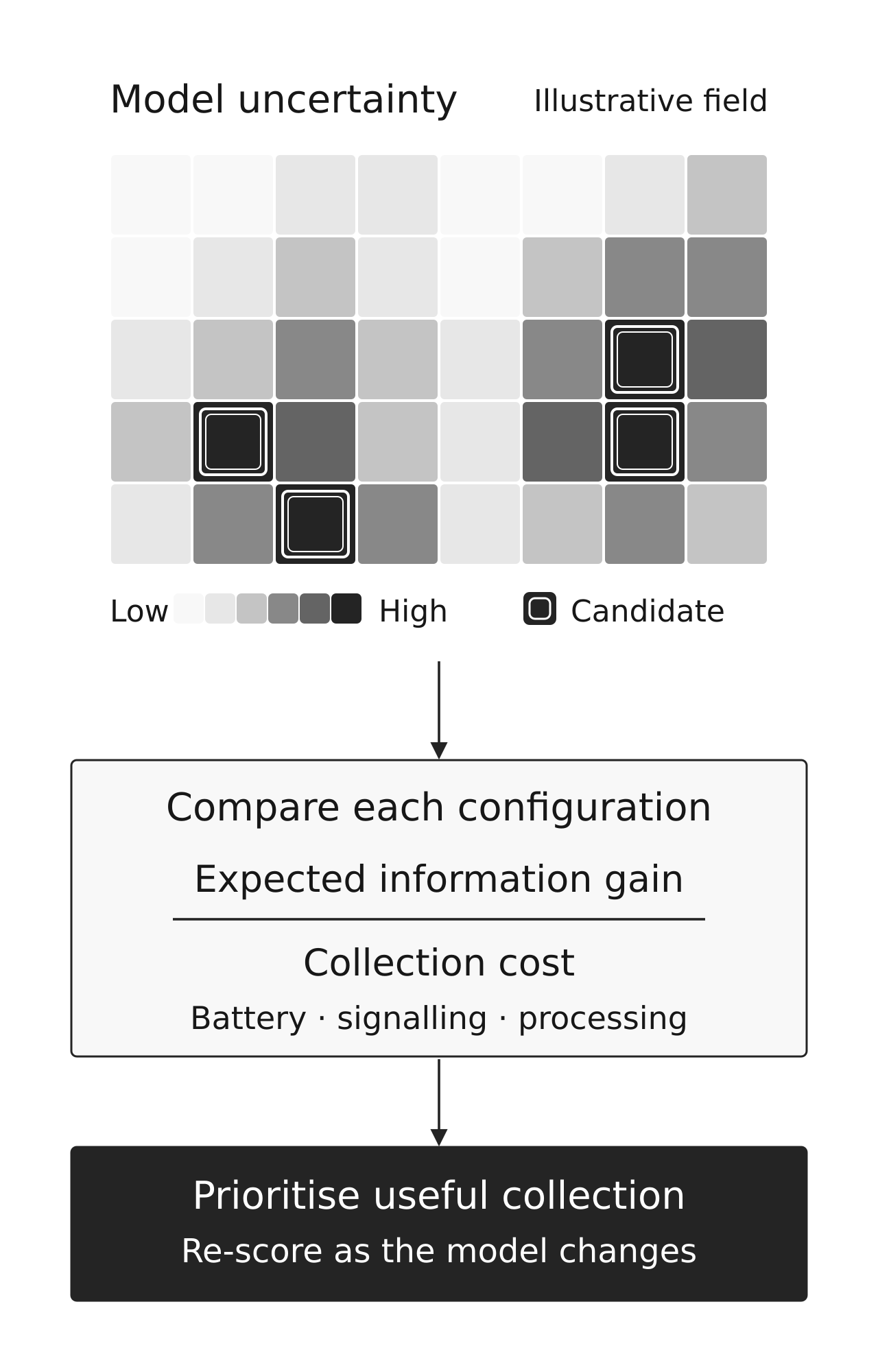
There is a well-known way to formalise this. If the model carries an explicit uncertainty, for example a predicted value with a confidence interval, then the value of a new measurement is the expected reduction of that uncertainty. This is the idea behind active learning and Bayesian experimental design, and it has been applied to sensor placement and environmental monitoring for decades. The RAN is a good fit because it already produces a spatial and temporal model of itself, and because the "sensors" are mobile and can be asked to measure on request.

Two things follow. First, the value of a measurement depends on what you already know, so it changes over time. Second, value has diminishing returns. The tenth measurement at a location is worth far less than the first.

Putting value and cost side by side

Once both sides are explicit, the strategy writes itself. For each candidate collection configuration, meaning a choice of which UEs or cells, which measurements, how often and for how long, estimate the expected information gain and the expected cost. Then prefer the configurations with the highest gain per unit cost.

This is different from uniform sampling, and it is also different from "collect where the KPIs are bad". Bad KPIs tell you a problem exists. High uncertainty tells you that you do not yet understand the problem well enough to fix it. They often overlap, but not always. A cell with poor throughput and a well-understood cause needs a fix, not more measurements.

The comparison also handles the trade between collection types. A short immediate MDT session on a few connected UEs and a long logged MDT campaign on many idle UEs produce very different data at very different cost. Scoring both on the same scale makes the choice explicit instead of habitual.

Knowing when to wait

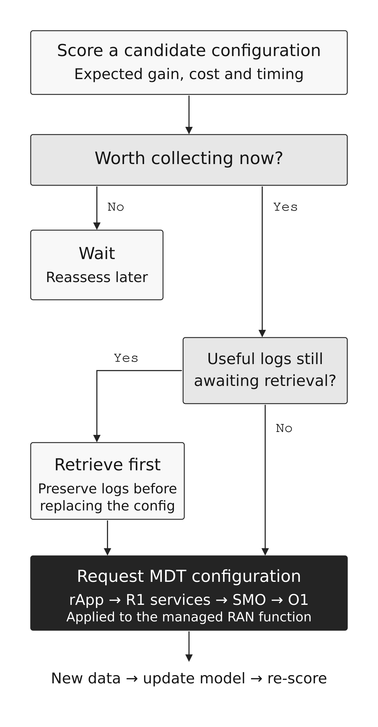
A cost-aware strategy has a second consequence that surprises people: sometimes the best action is no action. If the expected gain from a configuration does not cover its cost, do not apply it. If the decision that needs the data is not due for a week, there is no reason to spend UE battery today, especially if the model may learn what it needs from traffic that arrives on its own.

Waiting also protects data you already paid for. Logged MDT data sits at the UE until the network asks for it. Applying a new logged measurement configuration replaces the old one, and with it the log that was never retrieved. A strategy that only looks at what to collect next will quietly throw away what was collected last. Retrieval and reconfiguration belong in the same decision.

What this looks like as an rApp

This is a slow loop by nature. The model updates over hours, the uncertainty map changes over hours, and MDT configuration is a management operation carried out over O1. That places the function squarely in the Non-RT RIC as an rApp.

The inputs are what the SMO already has: performance data and trace data over O1, topology, and the model itself, which can be trained and managed through the Non-RT RIC AI/ML workflow services. The output is a trace and MDT configuration, requested through the RAN OAM services on R1 and applied by the SMO. Every time new data arrives, the model and its uncertainty are updated, and the next round of candidates is scored again.

The graphic on our research page shows the idea in one picture: an uncertainty field over an area, with the selected collection targets outlined where uncertainty is high. That is the whole loop, seen from above.

The practical payoff

Operators tend to care about three outcomes. Fewer measurement reports for the same model quality, which means less signalling and less UE battery drain. Faster convergence in areas that matter, because the samples go where they are informative. And a model that can say how sure it is, which turns a coverage map from a picture into something you can act on with a known risk.

The last point is the one we keep coming back to at EchoNest. A prediction without a confidence interval hides the question of whether to trust it. A prediction with one tells you whether to act, whether to measure first, or whether to wait. Collection is only the first place where that pays off.